SQLite Practice 1
Contents
SQLite Practice 1
Setup
Start by installing DB Browser for SQLite from here: https://sqlitebrowser.org/
Download DB File Here: https://github.com/ardhiraka/AlumVol1/blob/main/alum.db
Open DB File with DB Browser
Basics — SELECT, WHERE, ORDER BY
Exploring the data
Let’s take a quick look at the table before we filter it.
SELECT * selects every column in the table.
LIMIT 50 means we only get the first 50 rows.
SELECT *
FROM avocado
LIMIT 50
SELECT, WHERE, ORDER BY
We’re going to tackle these in one query.
The order of functions is essential in SQL. The order shown in these queries is generally the only order that works
SELECT
   date,
   avgprice,
   totalvol
FROM avocado
WHERE type = 1
ORDER BY totalvol DESC
SELECT
Here we define our columns via a comma separated list.
We can use * to select all columns in the table.
FROM
Here we define the table we want to pull the data from.
In this case, the name of the table is avocados.
WHERE
This is a filter. We can filter by any column in the table even if we haven’t selected it.
Multiple filters can be chained together using AND/OR.
ORDER BY
This sorts our data by the specified column.
We can specify ASCending or DESCending afterwards to change the order.
Using WHERE
Comparison Operators
We can use typical comparison operators with WHERE such as equals, greater than, less than etc.
These are standard symbols. You can see a full list here.
Contains
We can also use LIKE to find strings that contain a word.
We combine LIKE with a percent symbol to specify anything after or anything before.
The below query selects anything starting with ‘A’. We could put the percent sign before to find anything ending with ‘A’ (case-sensitive) or on both sides to find anything containing this character.
SELECT *
FROM avoregion
WHERE region LIKE 'A%'
Filtering with a list
One of the most commonly used functions with WHERE is IN which allows you to pass a list of items to filter by.
In the example below, we treat date as a string and pass 2 dates to filter.
We also combine this with a regionid filter.
SELECT *
FROM avocado
WHERE date IN ('2015-01-04','2015-01-11')
AND regionid=1
Working with Strings and Dates
Strings
String and Date syntax can vary a lot depending on which database management system you are using. In general, most of the string and date operations you can do in Excel are transferable to SQL but with different syntax.
SELECT
   UPPER(region)
 , SUBSTR(region,2,5)
 , SUBSTR(region,-3,3)
FROM avoregion
UPPER
This converts the text to uppercase.
This is very useful when used in conjunction with WHERE clauses if you are searching for a single word in text that is a mixture of cases.
SUBSTR
This takes a subsection of the string using the numbers we specify, the first indicates the character to start on and the second is the number of characters we take.
We can also use negative numbers to get the last characters.
Dates
When working with dates, the key is to make sure your data has the correct data type; it should be stored as an actual date.
If it isn’t you’ll need to either talk to your database administrator and get them to update the ‘create table’ statement to convert this.
In SQLite we can’t work with dates as easily, but the Syntax below will work in Postgres.
SELECT my_date,
 EXTRACT('year' FROM my_date) AS year,
 EXTRACT('month' FROM my_date) AS month,
 EXTRACT('day' FROM my_date) AS day,
 EXTRACT('hour' FROM my_date) AS hour,
 EXTRACT('minute' FROM my_date) AS minute,
 EXTRACT('second' FROM my_date) AS second,
 EXTRACT('decade' FROM my_date) AS decade,
 EXTRACT('dow' FROM my_date) AS day_of_week
FROM table_name
If in Postgres, you can also use the DATE_PART function
SELECT DATE_PART(‘year’, my_date) AS year
FROM table_name
Intermediate SQL — Aggregation, JOIN, UNION
Aggregation — SUM, AVG, MIN, MAX, GROUP BY
Let’s aggregate the data using the type column. We have 2 types, which at the moment are called ‘1’ and ‘2’. We’ll find out what those mean later. The order is also very important here. The GROUP BY must go at the end, and if we are using a WHERE, this should go before the GROUP BY.
SELECT
   type
 , AVG(avgprice)
 , SUM(totalvol)
FROM avocado
GROUP BY type
AVG
This takes the average of the column in brackets by row
SUM
This takes the sum of the column in brackets by row These aggregate functions are calculated over the rows selected which means we need to group the rows to get to what we want — the average or sum by type
GROUP BY This is the column we want to group by. SQL is performing the AVG or SUM calculation on all the rows within a group based on this function.
Other commonly used aggregations are MIN, MAX, COUNT.
Aggregate Filtering
Let’s say we want to take our previous example and filter out the types where the avgprice is less than 1.5.
Obviously there are only 2 types here so we could do this by eye but imagine we had hundreds!
We’ve already learnt to filter using WHERE but this won’t work to achieve what we want.
We can’t use WHERE with aggregate functions such as SUM and AVG because this will filter the underlying rows, not our summarised data.
Filtering the underlying data means we actually filter the individual rows and not our summary table. See the example below.
If we use WHERE, the AVG and SUM are now calculated using only rows with avgprice > 1.5.
Enter HAVING. This allows us to filter the aggregated rows after they’ve been calculated.
SELECT
   type
 , AVG(avgprice)
 , SUM(totalvol)
FROM avocado
GROUP BY type
HAVING AVG(avgprice) > 1.5
JOIN Theory
JOIN might be the single most important function in SQL. Understanding how joins work, in my opinion, takes you from a beginner to intermediate SQL user. In order to understand joins, you should understand the basics of relational databases and STAR schema tables. The first part of this guide gives a good explanation.
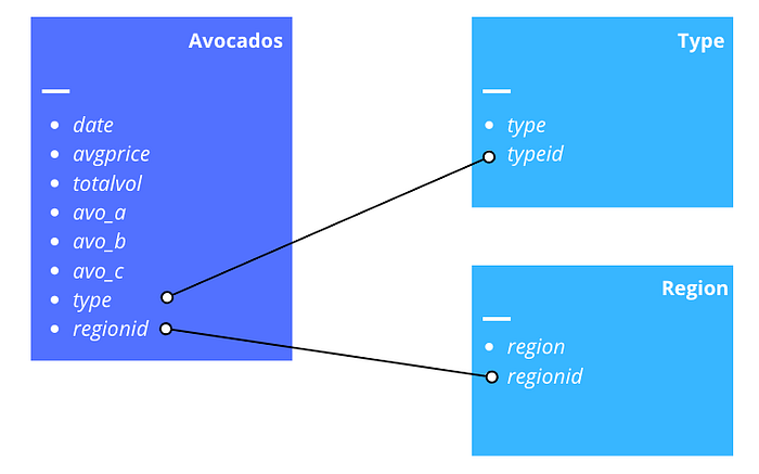
This is the schema of our set of tables. Without making joins we can’t get the actual type or region names because our Avocados table uses IDs in place of the actual names.
There are 4 main types of join; Inner, Outer, Left and Right. The differences are the rows that are kept in the joined table once the join is made.
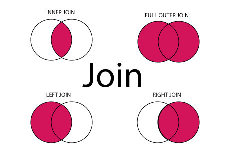
INNER JOIN: Returns all rows where there is at least one match in BOTH tables.
LEFT JOIN: Returns all rows from the left table and matched rows from the right table.
RIGHT JOIN: Returns all rows from the right table and matched rows from the left table.
FULL JOIN: Returns all rows where there is a match in ONE of the tables.
Consider a situation where a table has missing rows — eg if our Region table above was missing some region ids that were present in the main Avocado table.
In this situation, an INNER JOIN would cause us to lose any rows without a corresponding region id, so here we might want to use a left, right or outer join to keep all rows in the Avocado table.
It’s also worth noting that if there are duplicates in your dataset with the same ID, joining these will cause multiple lines to be created.
JOIN Composition

Specify the join type
Specify the table you are bringing on
After the ON, we name the columns
The order here doesn’t matter, if doing a LEFT JOIN, the left table is always the original table. The table you are bringing in is always the right table.
Specify the column
We put an equals sign between each column
This is the table you are joining to
This is the columns we are joining on. It should be equivalent to the table in ‘table1’ eg the same id.
You can use AND to join on multiple columns.
JOIN in SQL
We’ll just use left joins for the tutorial, but if you are following along, feel free to experiment with other join types.
SELECT *
FROM avocado
LEFT JOIN avotype ON avocado.type = avotype.typeid
We now have the columns typeid and type from the avo_type table. Let’s select only the date, avgprice and type columns.
Take a look at the query below, we’ve changed 2 parts of this query.
First, we’ve specified exactly which columns we’ll be using.
Then, tables have been given aliases.
We’ve called the avocados table ‘av’ and the avo_type table ‘avt’. We’ve also used these as an easy way to specify which columns to select. You’ll notice the type column is in both tables, so specifying which type we want is essential here.
SELECT
   av.date
 , av.avgprice
 , avt.type
FROM avocado av
LEFT JOIN avotype avt ON av.type = avt.typeid
UNION
Unions are used when we want to put one table on top of another. It isn’t really applicable for the data we have in this example, but I’ll show the syntax anyway.
In this query, we filter to type =1 and then use a union to stack this on top of a table for type !=1
Note that we’ve renamed the sum column here but the UNION still stacks it as it uses the position of the column and not the column name.
SELECT type, sum(totalvol) as totalvol
FROM avocado av
WHERE type = '1'
UNION
SELECT type, sum(totalvol) as t
FROM avocado av
WHERE type != '1'
Break Session
Go grab your coffee and chill for 15 min before we continue the session.
Advanced SQL
Exploring the Example Data
Let’s take a quick look at the table before we filter it.
SELECT *
FROM avocado
LIMIT 50
There are also 2 mapping tables in this dataset for type and regionid which map these numeric categories to their actual text.
JOIN as a Filter
By combining an INNER JOIN with a filter using AND, we can filter the table as we are joining it, providing a small performance boost over a regular join and WHERE filter. The is handy for big datasets but you’ll need to to know your data well as you may drop rows you didn’t intend to because this technique uses the INNER JOIN.
SELECT *
FROM avocado a
INNER JOIN avoregion b ON a.regionid = b.regionid
AND b.region = 'Denver'
Self Joins
Self joins are particularly useful when we need information in different rows to be in the same row. My dataset isn’t exactly set up to do this but we can still illustrate the point.
Let’s try to get the total volume for 2 regions on the same date on the same row.
First, note the aliases we’ve given to each avocados table. It’s the same table, but we’ve called each one a and b.
Inside the join, we’ve joined on date and regionid but we’ve used the does not equal operator (<>) to ensure we don’t join the same types together.
The result is a single row with both types on it, instead of each appearing in separate rows.
Please note, we do end up with duplicate data here as we have every combination of types. This could be avoided by filtering.
SELECT
  a.date, a.avo_a, a.type,
  b.avo_a, b.type, b.regionid
FROM avocado a
INNER JOIN avocado b
  ON a.date = b.date
  AND a.regionid=b.regionid
  AND a.type <> b.type
WHERE a.date = '2015-01-04'
  AND a.regionid = 1
CASE WHEN
CASE WHEN is essentially an IF function, which is found in almost all coding languages. As always, remember the ‘flow’: IF -> THEN -> ELSE when writing these.
We’ll use this to map types to the actual types (we could also do this with a join to our types table).
Note that the formula starts with CASE and ends with END. We can give the column an alias using AS after the END.
We can have as many WHEN/THEN clases as needed. Here we only need one because we have 2 types and the 2nd is covered by the ELSE
SELECT date, avo_a,
 CASE
  WHEN type =1 THEN 'conventional'
  ELSE 'organic'
 END AS avotype
FROM avocado
WHERE regionid = 1
Subqueries
A subquery is a nested query; it’s a query within a query Let’s say we want the full dataset but only for the top 10 regions by total volume.
We could find the top 10 with the query below, then we could use this list of regions to filter the main table. But what if we got new data and the top 10 changed? We’d have to run both queries again. We can make this more dynamic using a subquery.
To get the top 10, we’d run something like this:
SELECT b.region, ROUND(SUM(a.totalvol))
FROM avocado a
LEFT JOIN avoregion b ON a.regionid=b.regionid
GROUP BY 1
ORDER BY 2 DESC
LIMIT 1
In the query below, we use an INNER JOIN to filter the list to the regions in the subquery. We can also bring back data from the subquery because we’ve joined it.
Please note how aliases work here. The subquery aliases are independent of the main query aliases, which is why we have 2 ‘a’ and ‘b’ aliases. To refer to subquery columns we have to use the subquery alias which is c in this case.
SELECT date, totalvol, avo_a, avo_b, b.region, c.total_totalvol
FROM avocado a
LEFT JOIN avoregion b ON a.regionid=b.regionid
INNER JOIN (
  SELECT b.regionid, ROUND(SUM(a.totalvol)) as total_totalvol
  FROM avocado a
  LEFT JOIN avoregion b ON a.regionid=b.regionid
  GROUP BY 1
  ORDER BY 2 DESC
  LIMIT 10) c ON a.regionid = c.regionid
Subqueries can also be used after a FROM or WHERE clause. Let’s illustrate these with a simple example.
FROM Subquery
SELECT AVG(total_totalvol)
FROM (
  SELECT b.regionid, ROUND(SUM(a.totalvol)) as total_totalvol
  FROM avocado a
  LEFT JOIN avoregion b ON a.regionid=b.regionid
  GROUP BY 1
  ORDER BY 2 DESC
  LIMIT 10)
WHERE Subquery
SELECT *
FROM avocado
WHERE regionid IN (
  SELECT regionid
  FROM  avoregion
  WHERE region LIKE 'West%')
Common Table Expressions
A Common Table Expression (aka CTE, aka WITH statement) is a temporary data set to be used as part of a query. It only exists during the execution of that query; it cannot be used in other queries even within the same session
Common Table Expressions are recommended if you plan to reuse the subquery within the same query because the subquery is temporarily saved to memory, meaning it doesn’t need to be run multiple times. They generally also look much cleaner, so if you are sharing code it can be helpful for legibility.
In this example we’ll just use a CTE in a way that could also be done with a subquery and we’ll take the INNER JOIN example from above.
Here, we specify the subquery above our main query. We name it ‘top’ and specify the column names, then write a subquery. We can now call ‘top’ throughout the query to use this.
If we call it multiple types, SQL only has to generate the table once.
WITH top (regionid, total_totalvol) AS (
SELECT b.regionid, ROUND(SUM(a.totalvol))
  FROM avocado a
  LEFT JOIN avoregion b ON a.regionid=b.regionid
  GROUP BY 1
  ORDER BY 2 DESC
  LIMIT 10)

SELECT date, totalvol, avo_a, avo_b, b.region, top.total_totalvol
FROM avocado a
LEFT JOIN avoregion b ON a.regionid=b.regionid
INNER JOIN top ON a.regionid = top.regionid
Window Functions
A window function performs a calculation across a set of table rows that are somehow related to the current row. This is comparable to the type of calculation that can be done with an aggregate function. But unlike regular aggregate functions, use of a window function does not cause rows to become grouped into a single output row — the rows retain their separate identities. Behind the scenes, the window function is able to access more than just the current row of the query result.
Basically — we can use Window functions to look at rows above and below each row.
Running Total
The OVER ORDER BY sequence is the window function. OVER is almost like a GROUP BY, specifying how we want to construct our sum. The ORDER BY allows us to create the running total
SELECT
   date
 , avo_a
 , SUM(avo_a) OVER (ORDER BY date) AS running_total
FROM avocado
WHERE regionid =1 AND type =1
Total by date
Here, we use PARTITION BY to group the SUM by a given column (Date in this case)
SELECT
   date
 , avo_a
 , type
 , SUM(avo_a) OVER (PARTITION BY date) AS date_total
FROM avocado
WHERE regionid =1
Moving Average
This is where things start to heat up. By using AVG and ORDER BY date, we can specify ROWS to take a moving average. 3 PRECEDING is a 3 day moving average, but we can specify any number.
SELECT
   date
 , avo_a
 , AVG(avo_a) OVER (ORDER BY date ASC  ROWS 3 PRECEDING) AS date_total
FROM avocado
WHERE regionid =1 AND type=1
Get First Row
Let’s say we have varying end dates for each region. We can use Window Functions combined with a Subquery to get the first or last dates.
First, let’s define what our Subquery will be. The below query adds a row number, grouped by region id and ordered from most recent to oldest. We can select the first row from each grouping to get the newest date
SELECT
   date
   , regionid
   , ROW_NUMBER() OVER (PARTITION BY regionid ORDER BY date desc) AS row_number
FROM avocado
ORDER BY regionid
Now, we subquery the original and take only the first row.
SELECT date, regionid
FROM
  (SELECT
     date
     , regionid
     , ROW_NUMBER() OVER (PARTITION BY regionid
     ORDER BY date desc) AS row_number
  FROM avocado
  ORDER BY regionid)
WHERE row_number = 1